💻 Tutorial 01: Preparing your data for VIMuRe in python
VIMuRe v0.1.3 (latest)
If you use VIMuRe in your research, please cite (De Bacco et al. 2023).
TLDR: By the end of this tutorial, you should produce a data frame in the following format:
| ego | alter | reporter | tie_type | layer | weight |
|---|---|---|---|---|---|
| 103101 | 103201 | 103201 | borrowmoney | money | 1 |
| 101201 | 102901 | 102901 | borrowmoney | money | 1 |
| 111904 | 112602 | 111904 | lendmoney | money | 1 |
| 113201 | 104001 | 104001 | borrowmoney | money | 1 |
| 101303 | 115704 | 101303 | lendmoney | money | 1 |
| 112901 | 113601 | 113601 | borrowmoney | money | 1 |
| 104801 | 104901 | 104901 | borrowmoney | money | 1 |
| 108803 | 107503 | 108803 | lendmoney | money | 1 |
| 102901 | 103701 | 103701 | borrowmoney | money | 1 |
| 117202 | 115504 | 117202 | lendmoney | money | 1 |
Introduction
Before you start using VIMuRe, you need to prepare your data in a specific format. This tutorial will show you how to do that.
Here, we will illustrate the process of preparing data for the VIMuRe package using the “Data on Social Networks and Microfinance in Indian Villages” dataset (Banerjee et al. 2013b). This dataset contains network data on 75 villages in the Karnataka state of India.
⚙️ Setup
We will rely on the following packages in this tutorial:
import os

import pandas as pd
Step 1: Download edgelist
Follow the steps below to download the data.
- Click on this link to download the dataset from Prof. Matthew O. Jackson’s website 1. This will download a file called
IndianVillagesDataFiles.zipin your working directory. - Unzip the file. This will create a folder called
2010-0760_Datain your working directory. 💡 Tip: you can use theunzip()function from within R to unzip the file.
The folder structure should look like this:
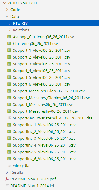
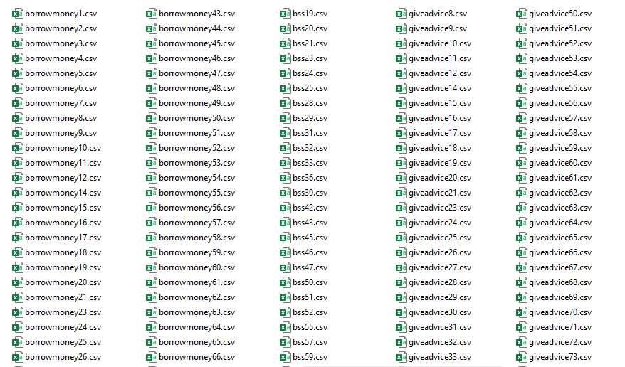
The data we need is within that Data/Raw_csv/ folder, and look like this:
Step 2: Collect individual-level metadata
We also need individual-level information metadata. This data is available on a separate source, the Harvard Dataverse (Banerjee et al. 2013a).
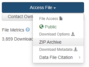
- Go to https://dataverse.harvard.edu/file.xhtml?fileId=2460959&version=9.4, read and accept the “License/Data Use Agreement” to gain access to the data. We are using version 9.4 of the dataset.
- Click on the “Access File” button, then “Download | ZIP Archive” to download the data.
- Unzip the file. This will create a folder called
datav4.0.zipin your working directory.
The data we need is within that datav4.0/Data/2. Demographics and Outcomes/ folder.
- Read the data into Python using the
pd.read_stata()function from pandas:
indivinfo = pd.read_stata("datav4.0/Data/2. Demographics and Outcomes/individual_characteristics.dta")
indivinfo.drop_duplicates(subset=["pid"], inplace=True) ## one individual (6109803) is repeated twice.- Ensure that the
pidis a string (we will need this later):
indivinfo["pid"] = indivinfo["pid"].astype(str)
indivinfo["hhid"] = indivinfo["hhid"].astype(str)
Step 3: Build an edge list per village
We will now build the edge list for each village. We will illustrate the process for village 1, but if you scroll down you will find the full script for all villages.
3.1. Read metadata
Let’s first subset the individual-level metadata to keep only the relevant village:
# Keep track of where the edgelist files are stored
RAW_CSV_FOLDER = "2010-0760_Data/Data/Raw_csv"

# Let's focus on just one village for now
selected_village = 1

# Filter the individual-level metadata to keep only the relevant village
resp = indivinfo[indivinfo["village"] == 1].copy()
resp["didsurv"] = 1The didsurv column is a dummy variable that indicates whether the individual participated in the survey. We will need this information later to tell our Bayesian model who participated in the survey.
3.2. Read village data
Now, let’s read the village_1.csv file and merge it with the individual-level metadata:
village_file = os.path.join(RAW_CSV_FOLDER, f"village{selected_village}.csv")
indiv = pd.read_csv(village_file, header = None, names=["hhid", "ppid", "gender", "age"])

## gender (1-Male, 2-Female)
indiv["gender"] = indiv["gender"].map({1: "Male", 2: "Female"})

## pre-process pid to match the format in the individual-level metadata
indiv["ppid"] = indiv["ppid"].astype(str)
indiv["hhid"] = indiv["hhid"].astype(str)
indiv["pid"] =  indiv.apply(lambda x: f'{x["hhid"]}{0 if len(x["ppid"]) != 2 else ""}{x["ppid"]}', axis=1)

## Select only the relevant columns
selected_cols = ["pid", "resp_status", "religion", "caste", "didsurv"]
indiv = pd.merge(indiv, resp[selected_cols], on="pid", how="left")
Which produces a dataframe that looks like this:
indiv.head()| hhid | ppid | gender | age | pid | resp_status | religion | caste | didsurv | |
|---|---|---|---|---|---|---|---|---|---|
| 0 | 1001 | 1 | Male | 75 | 100101 | nan | nan | nan | nan |
| 1 | 1001 | 2 | Female | 55 | 100102 | nan | nan | nan | nan |
| 2 | 1001 | 3 | Male | 24 | 100103 | nan | nan | nan | nan |
| 3 | 1001 | 4 | Female | 19 | 100104 | nan | nan | nan | nan |
| 4 | 1002 | 1 | Male | 38 | 100201 | Head of Household | HINDUISM | OBC | 1 |
3.3 Read reports per relationship type
The survey that produced this data collected information on a number of different types of relationships, four of which were “double sampled” (i.e., asked about in two ways, who people go to for that type of support, and who comes to them). Specifically, they asked about borrowing and receiving money, giving and receiving advice, borrowing and lending household items like kerosene and rice, and visiting and receiving guests. These distinct questions are represented in the data files with the following names:
- lendmoney,
- borrowmoney,
- giveadvice,
- helpdecision,
- keroricecome,
- keroricego,
- visitcome
- visitgo
Each of these relationships is stored in a separate file. For example, the file lendmoney1.csv contains information on who reported lending money to whom in village 1. We can read each of these files using the pd.read_csv() function.
First, we look over the data and specify an ALL_NA_CODES variable. This is a vector of all the codes that, after inspection, we identified were used to represent missing values in the data:
ALL_NA_CODES = ["9999999", "5555555", "7777777", "0"]We can then read in the data:
filepath_lendmoney = os.path.join(RAW_CSV_FOLDER, f"lendmoney{selected_village}.csv")
lendmoney = pd.read_csv(filepath_lendmoney, header=None, na_values=ALL_NA_CODES, dtype=str)
What the data look like
The data is stored here as a node list, but it will need to be further pre-processed as an edge list:
| 0 | 1 | 2 | 3 | 4 | 5 | 6 | 7 | 8 |
|---|---|---|---|---|---|---|---|---|
| 100201 | 107603 | nan | nan | nan | nan | nan | nan | nan |
| 100202 | 102902 | nan | nan | nan | nan | nan | nan | nan |
| 100601 | 101901 | 102601 | nan | nan | nan | nan | nan | nan |
| 100602 | 100501 | 101902 | nan | nan | nan | nan | nan | nan |
| 100701 | 100801 | 102101 | nan | nan | nan | nan | nan | nan |
Each row represents reports made by a single individual. The numbers in the first column are the pid (the “person identifier”) of the individual who reported the relationship. The remaining however many numbers listed in the same row are the pids of the individuals who were reported to be involved in the relationship.
3.4. Pre-process the data to build the edge list
We want the network data to be in the following format, plus a few additional columns:
| ego | alter |
|---|---|
| 100201 | 107603 |
| 100202 | 100201 |
| 100601 | 101901 |
| 100601 | 102601 |
| 100601 | 115501 |
| 100602 | 100501 |
| 100602 | 101902 |
| 100701 | 100801 |
| 100701 | 102101 |
| 100702 | 100801 |
To achieve this, we will need to pivot the data.
tie_type = "lendmoney"

# Example with the lendmoney data
edgelist_lendmoney = pd.melt(lendmoney, id_vars=[0]).dropna()
This produces a bogus variable column, which we can drop. We should also rename the columns to something more meaningful. It is important that we add a reporter column. This will be the pid of the individual who reported the relationship.
edgelist_lendmoney = edgelist_lendmoney.drop(columns="variable")\
       .rename(columns={0: "ego", "value": "alter"})\
       .assign(reporter=lambda x: x["ego"])

# Let's also add a column for the tie type
edgelist_lendmoney = edgelist_lendmoney.assign(tie_type=tie_type)

# Let's add a weight column too
edgelist_lendmoney = edgelist_lendmoney.assign(weight=1)
producing edgelist_lendmoney.head():
| ego | alter | reporter | tie_type | weight |
|---|---|---|---|---|
| 100201 | 107603 | 100201 | lendmoney | 1 |
| 100202 | 102902 | 100202 | lendmoney | 1 |
| 100601 | 101901 | 100601 | lendmoney | 1 |
| 100602 | 100501 | 100602 | lendmoney | 1 |
| 100701 | 100801 | 100701 | lendmoney | 1 |
So far, we only added tie_type = "lendmoney" to the data frame, but to make full use of VIMuRe, we also need to add the “flipped question” to the data frame, which in this case is tie_type = "borrowmoney". This is because the survey asked two different questions about borrowing and receiving money. The process is the same as before, except that we need to flip the ego and alter columns at the end.
There are also some other data cleaning steps that we need to perform: remove self-loops, remove duplicates and keep only reports made by registered reporters. We will do all of that inside a function in the next section, to make it easier to re-use.
4. Automating the process
4.1. Create a function to get the data for a given village and tie type
This function will also take care of the data cleaning steps that we described in the previous section. Importantly, it will also map the double-sampled tie types to the layer names we will use in VIMuRe.
Click here to expand the code for the get_karnataka_survey_data() function
def get_karnataka_survey_data(village_id: int, tie_type: str,
                              indivinfo: pd.DataFrame,
                              ties_layer_mapping={
                                  "borrowmoney": "money",
                                  "lendmoney": "money",
                                  "giveadvice": "advice",
                                  "helpdecision": "advice",
                                  "keroricego": "kerorice",
                                  "keroricecome": "kerorice",
                                  "visitgo": "visit",
                                  "visitcome": "visit",
                              },
                              all_na_codes=["9999999", "5555555", "7777777", "0"],
                              raw_csv_folder=RAW_CSV_FOLDER):
    """
    Read the raw data for a given tie type and village id,
    and return two dataframes: the edgelist and the list of respondents.

    Parameters
    ----------
    village_id : int
        The village id, between 1 and 10.
    tie_type : str
        The tie type
    indivinfo : pd.DataFrame
        The individual-level metadata
    all_na_codes : list, optional
        The list of codes that should be interpreted as missing values, by default ["9999999", "5555555", "7777777", "0"]
    raw_csv_folder : str, optional
        The path to the folder containing the raw csv files, by default "2010-0760_Data/Data/Raw_csv"

    Returns
    -------

    edgelist : pd.DataFrame
        The edgelist

    respondents : list
        The respondent metadata

    """

    # Filter the individual-level metadata to keep only the relevant village
    resp = indivinfo[indivinfo["village"] == village_id].copy()
    resp["didsurv"] = 1

    village_file = os.path.join(raw_csv_folder, f"village{village_id}.csv")
    metadata = pd.read_csv(village_file, header = None, names=["hhid", "ppid", "gender", "age"])

    ## gender (1-Male, 2-Female)
    metadata["gender"] = metadata["gender"].map({1: "Male", 2: "Female"})

    ## pre-process pid to match the format in the individual-level metadata
    metadata["ppid"] = metadata["ppid"].astype(str)
    metadata["hhid"] = metadata["hhid"].astype(str)
    metadata["pid"] =  metadata.apply(lambda x: f'{x["hhid"]}{0 if len(x["ppid"]) != 2 else ""}{x["ppid"]}', axis=1)

    ## Select only the relevant columns
    selected_cols = ["pid", "resp_status", "religion", "caste", "didsurv"]
    metadata = pd.merge(metadata, resp[selected_cols], on="pid", how="left")

    # Read the raw data
    filepath = os.path.join(raw_csv_folder, f"{tie_type}{village_id}.csv")
    df_raw = pd.read_csv(filepath, header=None, na_values=all_na_codes, dtype=str)

    # Example with the data
    edgelist = pd.melt(df_raw, id_vars=[0]).dropna()

    edgelist = edgelist.drop(columns="variable")\
          .rename(columns={0: "ego", "value": "alter"})\
          .assign(reporter=lambda x: x["ego"])

    # Let's also add a column for the tie type
    edgelist = edgelist.assign(tie_type=tie_type)

    # Let's add a weight column too
    edgelist = edgelist.assign(weight=1)

    # If the question was "Did you borrow money from anyone?", then we need to flip the ego and alter columns
    if tie_type in ["borrowmoney", "helpdecision", "keroricego", "visitgo"]:
        edgelist = edgelist.rename(columns={"ego": "alter", "alter": "ego"})

    edgelist["layer"] = edgelist["tie_type"].map(ties_layer_mapping)

    # Reorder the columns to make it easier to read
    edgelist = edgelist[["ego", "alter", "reporter", "tie_type", "layer", "weight"]]

    #### Further pre-processing steps ####

    # Who could actually report on the ties?
    reporters = set(metadata[metadata["didsurv"] == 1]["pid"])
    nodes = reporters.union(set(edgelist["ego"])).union(set(edgelist["alter"]))

    # Only keep reports made by those who were MARKED as reporters in metadata CSV
    edgelist = edgelist[edgelist["reporter"].isin(reporters)].copy()

    # Remove self-loops
    edgelist = edgelist[edgelist["ego"] != edgelist["alter"]].copy()

    # Remove duplicates
    edgelist.drop_duplicates(inplace=True)

    return edgelist, reporters
4.2 Getting an edgelist per layer
Each double-sampled tie type is mapped to a layer in VIMuRe. The mapping can be seen in the function we created above and is also shown below.
ties_layer_mapping={
    "borrowmoney": "money",
    "lendmoney": "money",
    "giveadvice": "advice",
    "helpdecision": "advice",
    "keroricego": "kerorice",
    "keroricecome": "kerorice",
    "visitgo": "visit",
    "visitcome": "visit",
}
Therefore, to get the edgelist for, say the money layer, we need to combine the borrowmoney and lendmoney tie types. We can do this by using the get_karnataka_survey_data function we created above.
# Get the edgelist for the money layer
edgelist_lendmoney, respondents =\
  get_karnataka_survey_data(village_id=1, tie_type="lendmoney", indivinfo=indivinfo)

edgelist_borrowmoney, _ = \
  get_karnataka_survey_data(village_id=1, tie_type="borrowmoney", indivinfo=indivinfo)

edgelist_money = pd.concat([edgelist_lendmoney, edgelist_borrowmoney], axis=0)
which now gives us all the edges for the money layer:
edgelist_money.sample(n=10, random_state=1)| ego | alter | reporter | tie_type | layer | weight | |
|---|---|---|---|---|---|---|
| 235 | 103101 | 103201 | 103201 | borrowmoney | money | 1 |
| 229 | 101201 | 102901 | 102901 | borrowmoney | money | 1 |
| 130 | 111904 | 112602 | 111904 | lendmoney | money | 1 |
| 40 | 113201 | 104001 | 104001 | borrowmoney | money | 1 |
| 14 | 101303 | 115704 | 101303 | lendmoney | money | 1 |
| 345 | 112901 | 113601 | 113601 | borrowmoney | money | 1 |
| 50 | 104801 | 104901 | 104901 | borrowmoney | money | 1 |
| 97 | 108803 | 107503 | 108803 | lendmoney | money | 1 |
| 241 | 102901 | 103701 | 103701 | borrowmoney | money | 1 |
| 198 | 117202 | 115504 | 117202 | lendmoney | money | 1 |
The above is the format we want the data to be in! This format will make it easier to work with VIMuRe. Although, only the ego, alter, reporter columns are required. The tie_type, layer and weight columns are optional, but useful to have.
Use the full pre-processing script below to pre-process all the data for all tie types and save it to a single vil1_money.csv file. We also save the reporters list to, as a data frame, to a vil1_money_reporters.csv file.
Click to see full pre-processing script
import os
import pandas as pd

# village IDs 13 and 22 are missing
VALID_VILLAGE_IDS = [i for i in range(1, 77+1) if i != 13 and i != 22]

RAW_CSV_FOLDER = "2010-0760_Data/Data/Raw_csv"

ties_layer_mapping={
    "borrowmoney": "money",
    "lendmoney": "money",
    "giveadvice": "advice",
    "helpdecision": "advice",
    "keroricego": "kerorice",
    "keroricecome": "kerorice",
    "visitgo": "visit",
    "visitcome": "visit",
}

def get_karnataka_survey_data(village_id: int, tie_type: str,
                              indivinfo: pd.DataFrame,
                              ties_layer_mapping=ties_layer_mapping,
                              all_na_codes=["9999999", "5555555", "7777777", "0"],
                              raw_csv_folder=RAW_CSV_FOLDER):
    """
    Read the raw data for a given tie type and village id,
    and return two dataframes: the edgelist and the list of respondents.

    Parameters
    ----------
    village_id : int
        The village id, between 1 and 10.
    tie_type : str
        The tie type
    indivinfo : pd.DataFrame
        The individual-level metadata
    all_na_codes : list, optional
        The list of codes that should be interpreted as missing values, by default ["9999999", "5555555", "7777777", "0"]
    raw_csv_folder : str, optional
        The path to the folder containing the raw csv files, by default "2010-0760_Data/Data/Raw_csv"

    Returns
    -------

    edgelist : pd.DataFrame
        The edgelist

    respondents : list
        The respondent metadata

    """

    # Filter the individual-level metadata to keep only the relevant village
    resp = indivinfo[indivinfo["village"] == village_id].copy()
    resp["didsurv"] = 1

    village_file = os.path.join(raw_csv_folder, f"village{village_id}.csv")
    metadata = pd.read_csv(village_file, header = None, names=["hhid", "ppid", "gender", "age"])

    ## gender (1-Male, 2-Female)
    metadata["gender"] = metadata["gender"].map({1: "Male", 2: "Female"})

    ## pre-process pid to match the format in the individual-level metadata
    metadata["ppid"] = metadata["ppid"].astype(str)
    metadata["hhid"] = metadata["hhid"].astype(str)
    metadata["pid"] =  metadata.apply(lambda x: f'{x["hhid"]}{0 if len(x["ppid"]) != 2 else ""}{x["ppid"]}', axis=1)

    ## Select only the relevant columns
    selected_cols = ["pid", "resp_status", "religion", "caste", "didsurv"]
    metadata = pd.merge(metadata, resp[selected_cols], on="pid", how="left")

    # Read the raw data
    filepath = os.path.join(raw_csv_folder, f"{tie_type}{village_id}.csv")
    df_raw = pd.read_csv(filepath, header=None, na_values=all_na_codes, dtype=str)

    # Example with the data
    edgelist = pd.melt(df_raw, id_vars=[0]).dropna()

    edgelist = edgelist.drop(columns="variable")\
          .rename(columns={0: "ego", "value": "alter"})\
          .assign(reporter=lambda x: x["ego"])

    # Let's also add a column for the tie type
    edgelist = edgelist.assign(tie_type=tie_type)

    # Let's add a weight column too
    edgelist = edgelist.assign(weight=1)

    # If the question was "Did you borrow money from anyone?", then we need to flip the ego and alter columns
    if tie_type in ["borrowmoney", "helpdecision", "keroricego", "visitgo"]:
        edgelist = edgelist.rename(columns={"ego": "alter", "alter": "ego"})

    edgelist["layer"] = edgelist["tie_type"].map(ties_layer_mapping)

    # Reorder the columns to make it easier to read
    edgelist = edgelist[["ego", "alter", "reporter", "tie_type", "layer", "weight"]]

    #### Further pre-processing steps ####

    # Who could actually report on the ties?
    reporters = set(metadata[metadata["didsurv"] == 1]["pid"])
    nodes = reporters.union(set(edgelist["ego"])).union(set(edgelist["alter"]))

    # Only keep reports made by those who were MARKED as reporters in metadata CSV
    edgelist = edgelist[edgelist["reporter"].isin(reporters)].copy()

    # Remove self-loops
    edgelist = edgelist[edgelist["ego"] != edgelist["alter"]].copy()

    # Remove duplicates
    edgelist.drop_duplicates(inplace=True)

    return edgelist, reporters

def get_layer(village_id, layer_name, indivinfo,
              raw_csv_folder=RAW_CSV_FOLDER):

    tie_types = {
        "money": ["lendmoney", "borrowmoney"],
        "advice": ["giveadvice", "helpdecision"],
        "kerorice": ["keroricego", "keroricecome"],
        "visit": ["visitgo", "visitcome"],
    }

    selected_tie_types = tie_types[layer_name]

    edgelist = pd.DataFrame()
    reporters = set()

    for tie_type in selected_tie_types:
        edgelist_, reporters_ = get_karnataka_survey_data(village_id=village_id,
                                                            tie_type=tie_type,
                                                            indivinfo=indivinfo,
                                                            raw_csv_folder=raw_csv_folder)
        edgelist = pd.concat([edgelist, edgelist_])
        reporters = reporters.union(reporters_)

    return edgelist, reporters


indivinfo = pd.read_stata("datav4.0/Data/2. Demographics and Outcomes/individual_characteristics.dta")
indivinfo.drop_duplicates(subset=["pid"], inplace=True) ## one individual (6109803) is repeated twice.
indivinfo["pid"] = indivinfo["pid"].astype(str)
indivinfo["hhid"] = indivinfo["hhid"].astype(str)


for i in VALID_VILLAGE_IDS:
    for layer_name in ["money", "advice", "kerorice", "visit"]:
      print(f"Processing village {i}")
      edgelist, reporters = get_layer(village_id=i,
                                        layer_name=layer_name,
                                        indivinfo=indivinfo,
                                        raw_csv_folder=RAW_CSV_FOLDER)
      edgelist.to_csv(f"vil{i}_{layer_name}.csv", index=False)
      # save reporters to a separate file
      pd.DataFrame({"reporter": list(reporters)}).to_csv(f"vil{i}_{layer_name}_reporters.csv", index=False)

    print(f"Done with village {i}")
References
Footnotes
Note that the authors provide a different version of the network data on Harvard Dataverse (Banerjee et al. 2013a). However, we will use the raw version provided by Prof. Jackson in this tutorial, as the version of the Dataverse has already had some pre-processing (importantly, they have made the adjacency matrices symmetric), while the version provided by Prof. Jackson gives the original node list. We will use the Harvard Dataverse files just for the metadata.↩︎